Uncertainty in Sea Ice Thickness Uncertainties
By Alek Petty
alekpetty.com / @alekpetty
The Arctic and Southern Oceans are typically covered by a relatively thin layer of ice – sea ice – that waxes and wanes with the seasons. Sea ice that’s only a few weeks old might typically be an inch or two thick, semi-transparent and supple. As snow begins to accumulate and the ice thickens, strengthens and deforms through winter, it starts to resemble a more characteristic ‘pack’ of conjoined bright-white ice floes.
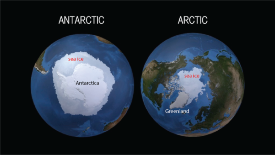
Figure 1: Maps of the Antarctic (left) and Arctic (right) including the floating sea ice component of our cryosphere. Adapted from a NASA SVS image.
Summer Arctic sea ice coverage – the fraction of the Arctic Ocean covered by ice – has roughly halved since the 1980s, while Southern Ocean sea ice has only more recently experienced a sharp decline. The decrease in Arctic sea ice especially has contributed to a well known positive feedback loop of polar amplification – the bright ice is replaced by a darker open ocean surface, increasing the warming and further loss of ice. Loss of sea ice is also disrupting key ocean circulation pathways and fundamentally altering the biogeochemical balance of our polar oceans. Sea ice decline is not just a victim of climate change, but an active participant.
Satellite monitoring of sea ice coverage across both hemispheres is now relatively routine (thanks NASA!). Routine satellite monitoring of ice thickness, however, still has a ways to go. For one, only in the last couple of decades have we had satellites at our disposal capable of estimating sea ice thickness. Secondly, measuring sea ice thickness from these new satellites is tricky. This challenge is what I want to talk to you about in this blog post. Not just the challenge of estimating sea ice thickness, but also the challenge of determining how uncertain our thickness estimates might be.
The first thing to note about measuring sea ice thickness from space is that the instruments we use to do this don’t actually measure sea ice thickness. The instruments are altimeters which measure the time of flight of radar or laser pulses that bounce off the Earth’s surface and convert that travel time to distance, or a height above some reference surface (e.g. the Earth’s ellipsoid). The height of the sea ice surface is then differenced from the height of the local sea level to derive an estimate of sea ice freeboard.
ICESat-2 is NASA’s big new fancy laser altimeter that profiles the Earth’s surface elevation with incredible resolution (~10 m footprints) and high precision (less than an inch!). ESA launched the CryoSat-2 radar altimeter over 10 years ago, which is still going strong today. Both ICESat-2 and CryoSat-2 altimeters each employ their own bespoke algorithms to distinguish height returns between ice and open ocean (sea level) surfaces that I won’t go into right now. Difference the two height measurements (after some more fancy processing steps) and you get freeboard (see Figure 1).
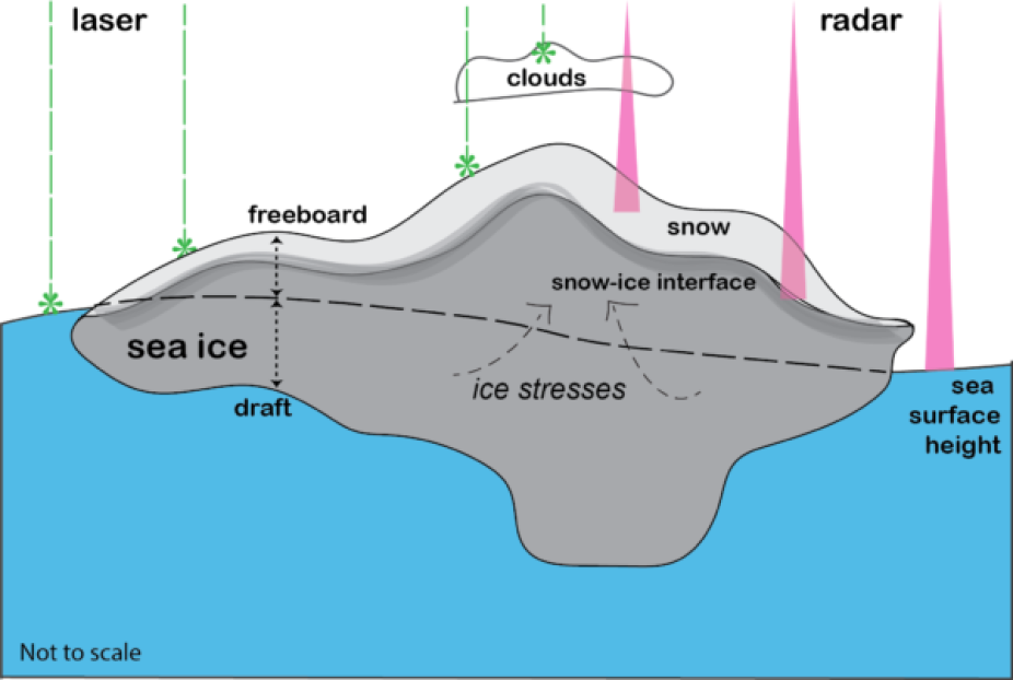
Figure 2: A simplified schematic of sea ice and how we measure sea ice thickness from space using either radar or laser altimetry of sea ice freeboard. Some of the key areas of complexity involved in this approach are highlighted. The sea ice floe depicted is not to scale. Sea ice is generally much thinner/broken up and spread out than depicted here!
How do we go from freeboard measurements to thickness estimates? The first big assumption we generally make is that the ice is in ‘hydrostatic equilibrium’ which is a fancy way of saying the ice is freely floating and the displacement of water can be related to the relative density difference between the ice (including its overlying snow cover) and the seawater its displacing. Remember learning about Archimedes and his bathtub ‘Eureka!’ moment in school? Same concept.
Assuming the ice is freely floating we can then very easily convert the freeboard measurement to thickness using an equation that relates the ice thickness to the measured freeboard, as well as the overlying snow depth, snow density, sea ice density and the displaced sea water density. The equations change slightly depending on whether we measure total freeboard (the height of the ice plus snow above sea level) as we do with laser altimeters like ICESat-2, or just the ice freeboard, as we think we do with the radar altimeters like CryoSat-2 (see Figure 2). NB: some other methods exist for inferring sea ice thickness from different, generally passive, sensors, but i’m not going to talk about that here!.
Where does all this extra information come from? The density of seawater we know pretty well by now (!) and thankfully it doesn’t change all that much (it’s around 1024 kg/m3). The other variables are a bit trickier. Estimates of Arctic snow depth and density have generally relied on a 50 year-old snow climatology produced from Soviet-era drifting field stations. Pretty cool data, but also pretty outdated. More recent studies have attempted to model snow accumulation over sea ice instead – using snowfall estimates from weather models and tracking the movement of ice and snow parcels around the Arctic. While these models are expected to be more representative of current conditions, they are still models, and models without much data to constrain them. We somehow know even less about Southern Ocean snow conditions.
Sea ice density is generally estimated based on information collected by sporadic field campaigns and heated discussions in the community (some say 900 kg/m3, others say 915 kg/m3, some go as high as 916 kg/m3 just to be awkward). Put that information all together and we can finally estimate sea ice thickness! But hold on (says reviewer 2, probably) – what about the thickness ‘uncertainty’?! Well as I said earlier, that’s where things arguably get even harder…
There are always different expectations of uncertainty quantification, which differ wildly based on the specific discipline you happen to be working in and the types of data and approaches that are typical in your community. Understanding these differences is a primary goal of the CLIVAR Ocean Uncertainty Quantification working group hosting this blog!
In cases where direct observations of the given variable are plentiful (damn you!), the uncertainty can generally be estimated by comparing the derived variable against the direct observations and looking at the spread and/or bias between the two. Simple! Unfortunately, we don’t have many direct observations of Arctic or Southern Ocean sea ice coincident with our satellite observations. Sea ice is very far away, and it moves, so taking ground-truth measurements of data collected by satellites is very challenging – you really need to be at the exact right place at the exact right time and, again, it’s very far away. And cold. Some brave souls have managed to do this, which has been hugely beneficial to the community, but the data are sporadic at best. There have also been some cool efforts to collect coincident airborne measurements, but these are still pretty limited and the data isn’t exactly ground-truth. Upward looking sonar moorings anchored to the deep ocean seabed and collected on a semi-annual basis are also particularly helpful, but they are (currently) stationary and thus only profile the region where they are deployed.
So instead we have to get a bit more creative. A common approach in the sea ice altimetry community is to ‘propagate’ uncertainties from all the various input assumptions we discussed in the previous paragraph (take partial derivatives of all the terms in the hydrostatic equilibrium thickness equation). The individual uncertainty estimates are also typically divided into ‘random’ and ‘systematic’ uncertainty contributions as follows:.
Random uncertainties can be thought of as a form of noise we have no real hope of capturing in our observations/models. The nice thing about random errors is that we generally assume the uncertainties are uncorrelated with each other, so the aggregated uncertainty quickly reduces with the number of observations we combine together (e.g. when averaging). So when we produce, for example, a 100 km gridded mean that involves thousands of observations, we assume the mean error reduces to a very low/near-zero value. Historically, studies have focused mainly on understanding thickness at just the very large/basin-scales, so they would ignore such sources uncertainties. As we try and keep up with the advances in satellite altimetry and move towards producing thickness estimates at very local-scales (meters instead of kilometers!), random uncertainties can no longer be ignored.
Systematic uncertainties can be thought of as biases acting in a certain direction which we can (potentially, one day) do something about. They might indicate a problem in the observations we are taking, e.g. our sensor may have a calibration issue and may not be tracking the sea ice surface incorrectly. Alternatively, we might be making incorrect assumptions in some of the input variables needed to convert freeboard to thickness, e.g. we might be assuming snow is thinner than it actually is. Systematic uncertainties don’t reduce with the number of observations we include in an average, so they dominate the uncertainty when we talk of things like ‘mean Arctic sea ice thickness uncertainty’.
How do we go about calculating these individual uncertainties? Random uncertainty we can estimate to some degree from the known errors of our individual measurement approaches, e.g. the precision of our instrument. Additional contributions include small-scale variability of snow depth, snow density and ice density that we don’t expect our models (or basic estimates in the case of ice density) to be able to capture.
Systematic uncertainties can be even more challenging to prescribe. The primary source of uncertainty for freeboard is uncertainty in our estimate of local sea level, which depends on the density and size of cracks (commonly referred to as leads) in the ice pack which we need to determine sea level. In areas of high ice concentration, leads can be few and far between, drastically increasing the sea level height and thus freeboard uncertainty. For all the additional input assumptions (e.g. snow depth/density), the typical approach taken is to estimate uncertainty from the spread of possible input assumptions available – e.g. the spread in model estimates of snow depth or density. The difficulty here is that there is a lot of subjectivity involved in choosing these assumptions and calculating the spread. Do we include everything we’ve ever heard of or only select assumptions we think of as ‘reasonable’? A last resort is to just…guess (we would call this a heuristic uncertainty estimate to disguise the fact we’re just guessing).
And what about the basic assumption we discussed earlier about the ice being freely floating? Some very limited evidence (there’s a pattern here) has suggested that at very local scales this assumption can break down – the ice is moving and/or deforming (note the internal ice stresses in Figure 2) and is not freely floating, which could contribute up to a half meter of error to our thickness estimate according to some studies. But those studies also suggest that this is a highly local issue and that when looking at the large scale (kilometers) we are probably safe to assume this assumption is valid and any systematic bias this introduces becomes negligible. This could also be considered (I think!) as a type of ‘representation error’, which was discussed more in Kyla Drushka’s blog in this same series of articles.
The point of all this is that we could measure height really accurately – as we think we can now do with these new fancy satellite altimeters – but uncertain knowledge of other key variables, and uncertainty in how best to estimate our uncertainties (!) continues to pose a real challenge to further progress.
To show some numbers and to give (very keen!) readers a chance to play around with these ideas more, I created a Jupyter Notebook to describe the conversion of ICESat-2 sea ice freeboard (ATL10, https://nsidc.org/data/atl10) to sea ice thickness including estimates of sea ice thickness uncertainties. Please check it out here: https://github.com/akpetty/thickness_uncertainity/blob/main/thickness_uncertainity_demo.ipynb. In this example the thickness ranges from 0 to 8 m (mean of ~2 m) while the total uncertainty varies from 0.8 to 1.4 m, or around 20 to 50% (!) of the total thickness. So, quite uncertain in general.
I want to conclude with some thoughts on what might be needed to move the science forward. I would love to hear suggestions on these or any other points in the comments below:
- More ground-truth data – Targeted field campaigns that can somehow cover a large area at the same time the satellite overpasses. These need to be highly coordinated with the satellite altimeter community and provide measurements similar to the satellite measurements/input assumptions (e.g. same spatial scales). Autonomous vehicles could provide the key breakthrough here in the coming decades.
- Better community agreement – Better agreement on the various uncertainty contributions and communication standards. Combined expert knowledge might be our only realistic short-term option for constraining uncertainty.
- More sophisticated uncertainty calculations – Explore new methods for estimating uncertainties (e.g. Monte Carlo methods, Bayesian approaches). There have been some encouraging studies doing this but there are computational demands that need to be overcome.
- Deeper understanding of sea ice uncertainties – Is a random/systematic uncertainty differentiation the best approach? How correlated are the uncertainties in space and with each other? How can we hope to figure this out?
Finally, it is worth reiterating that the fact we can even measure height to centimeter-level precision from satellites 500 km away is a truly great accomplishment – the result of several decades worth of hard work from the sea ice altimetry community. Converting these heights to estimates of freeboard and thickness is always going to be a challenge, but better understanding and constraining our current window of uncertainty is needed to fully realize the primary challenges that need to be overcome.